
Read epithelial architecture before measuring thickness
Epithelial tissue forms closely connected sheets at surfaces and glands. The apical domain faces a lumen or exterior, lateral surfaces contact neighboring cells, and the basal domain attaches to a basement membrane. Underlying connective tissue supplies support and exchange; an epithelial sheet itself lacks blood vessels. A lumen can be continuous with the exterior even when it lies deep inside the body, so “inside the organ” and “inside the body’s internal fluid compartment” are different boundaries.
Learning outcome: Inspect the real epithelial image and retain two visible features and one uncertain feature. Compare model angles 0° and 60° without changing thickness. Explain why nuclear rows and apparent width cannot alone distinguish simple from stratified tissue.
Starting recap
Use subject-relative anatomical directions, actual licensed tissue images, compartment conservation and explicit feedback/system boundaries; distinguish structural evidence from functional and clinical claims.
All lessons are open directly. Your saved experiments remain when you leave and return.
Try
A true perpendicular thickness of 20 μm with a 60° path gives 20/cos60°=40 μm. The sheet has not doubled its true thickness. At normal incidence the path is 20 μm.
Open the experimentPredict
Can two differently oriented sections of an unchanged sheet show different apparent path lengths?
Experiment
Inspect the real epithelial image and retain two visible features and one uncertain feature. Compare model angles 0° and 60° without changing thickness. Explain why nuclear rows and apparent width cannot alone distinguish simple from stratified tissue.
Separate epithelial thickness from section orientation
Worked teaching model · synthetic values · Ideal parallel slab, path length t/cos θ, no tissue distortion. The actual image supplies architecture, not this synthetic thickness or angle. Nuclear positions alone do not count cell layers.
Reset keeps your prediction, captures and practice history.
A longer oblique path need not mean a thicker epithelial layer.
The ideal geometry controls path length only. Histological cell-layer classification additionally needs apical/basal boundaries and cell contacts; preparation distortion and section orientation complicate an actual image.
| Quantity | Value | Unit |
|---|---|---|
| True normal thickness | 20 | μm |
| Oblique path length | 40.00000 | μm |
| Path-to-normal ratio | 2.000000 | ratio |
Original bounded models, not measurements of the accompanying actual micrographs or any person. Retain settings, predictions and limitations in the notebook.
A longer oblique path need not mean a thicker epithelial layer.
The ideal geometry controls path length only. Histological cell-layer classification additionally needs apical/basal boundaries and cell contacts; preparation distortion and section orientation complicate an actual image.
Captures preserve recipes and replay their calculated results. They are synthetic model evidence, not physical measurements.
Understand
1. Define the structure and boundary
Epithelial tissue forms closely connected sheets at surfaces and glands. The apical domain faces a lumen or exterior, lateral surfaces contact neighboring cells, and the basal domain attaches to a basement membrane. Underlying connective tissue supplies support and exchange; an epithelial sheet itself lacks blood vessels. A lumen can be continuous with the exterior even when it lies deep inside the body, so “inside the organ” and “inside the body’s internal fluid compartment” are different boundaries.
2. Connect anatomical evidence and mechanism
Simple epithelium is one cell layer; stratified epithelium has multiple layers and is named by its superficial cell shape. Squamous cells are flattened, cuboidal cells roughly as tall as wide, and columnar cells taller than wide. Pseudostratified epithelium can show nuclei at several heights although its cells contact the basement membrane; not all reach the free surface. Transitional epithelium changes apparent shape with distension. A row of nuclei is not a reliable independent count of cell layers.
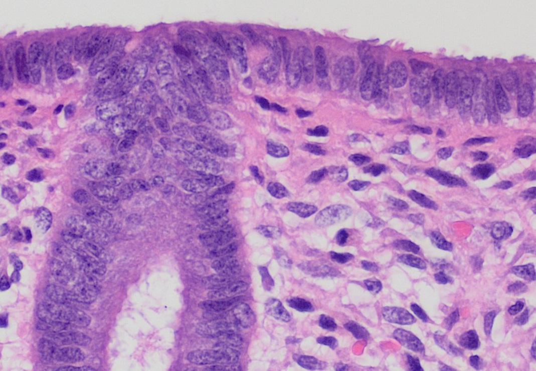
The supplied actual CC0 endometrial micrograph shows a surface border of columnar cells and underlying tissue, with a curved gland profile on the left. Trace the free surface across the top, locate the epithelial band and distinguish it from the less orderly underlying cell arrangement. Record features you can see before opening the source identity. Do not infer pathology, hormonal state or exact cell boundaries from this single educational field. Tissue preparation, oblique sectioning and optical overlap can obscure contacts.
Our separate ideal slab model makes a measurement ambiguity explicit. A path through parallel surfaces at angle θ from the normal travels t/cos θ for true perpendicular thickness t. A long oblique path need not indicate a thicker sheet. These numerical thicknesses are invented, not extracted from the micrograph; the displayed image has no calibrated scale bar for this exercise. Cell polarity and junctions support selective barriers and directional secretion, but morphology alone does not measure permeability.
Observe actual tissue images before accepting a label
These are actual published micrographs, not generated images or the numerical model’s invented measurements. Retain two visible features, a tentative tissue class and one unresolved feature in your lesson notebook. The accessible descriptions supply equivalent observations; using them or the public source label is guided evidence, not a blinded identification test.
Compare source identity, visible evidence and limits
Source identifies normal simple columnar endometrial epithelium. The continuous tall-cell surface supports columnar architecture; nuclei at differing heights and curved profiles do not alone prove multiple layers. This is source-labeled guided practice, not a pathological or hormonal diagnosis.
Mikael Häggström; 9 April 2022. Source and file history · CC0 1.0 dedication · Download unchanged image. Checked 30 October 2026. No endorsement or diagnostic use is implied.

Download exact source, license, dimensions and SHA-256 provenance. For independent practical evidence, a qualified reviewer must supply a genuinely unfamiliar licensed specimen/image and assess identification, uncertainty and reasoning; viewing these labeled examples does not fulfill that gate.
3. Audit an original worked comparison
A true perpendicular thickness of 20 μm with a 60° path gives 20/cos60°=40 μm. The sheet has not doubled its true thickness. At normal incidence the path is 20 μm.
4. Predict and investigate
Predict first: Can two differently oriented sections of an unchanged sheet show different apparent path lengths?
Inspect the real epithelial image and retain two visible features and one uncertain feature. Compare model angles 0° and 60° without changing thickness. Explain why nuclear rows and apparent width cannot alone distinguish simple from stratified tissue.
5. Transfer to a changed case
Apply the mechanism to a changed boundary
An ideal 30 μm slab is crossed at 60° from its normal. What path length is seen, and what additional evidence is needed to count layers?
Retain the first response, units, uncertainty and any prior feedback exposure in the notebook before comparing this public explanation.
Compare a worked response
The path is 60 μm. Layer classification needs cell contacts with basal and apical surfaces or additional well-oriented sections, not only path length or nuclear positions.
6. Retain an evidence-based defense
Use the Anatomy and Physiology course workspace to preserve original reasoning, actual image observations with uncertainty, model settings and a reviewer-supplied new transfer. Public feedback is guided practice, not independent mastery or clinical assessment. No examination, personal health data, specimen collection or physiological challenge is requested.
Supporting anatomical mechanism, checked 30 October 2026. Numerical packets and diagrams are original teaching models; actual tissue images have separate attribution, download and CC0 provenance records.
Apply
Public practice checks a specific claim. It does not establish independent mastery.
An ideal 30 μm slab is crossed at 60° from its normal. What path length is seen, and what additional evidence is needed to count layers?
Continue
Completion requires a saved prediction, at least one capture and a reflection. Presence checks do not grade your reasoning.
Skipping retains experiments and awards no mastery.
Save a science backup or import one
Science work is stored locally in this browser, separately from mathematics and AI. It does not sync automatically. Use this science-only backup; this checkout's older all-subject export does not include science.
A legacy file is available only when the complete snapshot fits the 36 MB limit. For larger snapshots, prepare a complete file set below; never discard notebooks to make a smaller file.
Matching imported notebook drafts replace their current drafts. Omitted lessons and known first attempts remain. Export your current work first if you want to retain both drafts.
Complete file sets and course backups
A file set can hold more work than one science file. Keep its manifest and every part together. Each file is limited to 36 MB. This format needs this version of LearnAI or a compatible newer version; older versions can use only the legacy single-file backup above.
The set includes every saved science course and global continuation at this moment. Later edits need a new export. A conflicting tab exports its own visible work, which may differ from saved work in another tab.
0 file(s) selected. File order and filenames do not determine identity. Missing, changed or conflicting parts block the entire restore; no good part is applied by itself.
Science storage: loading. No account or remote computation is required.